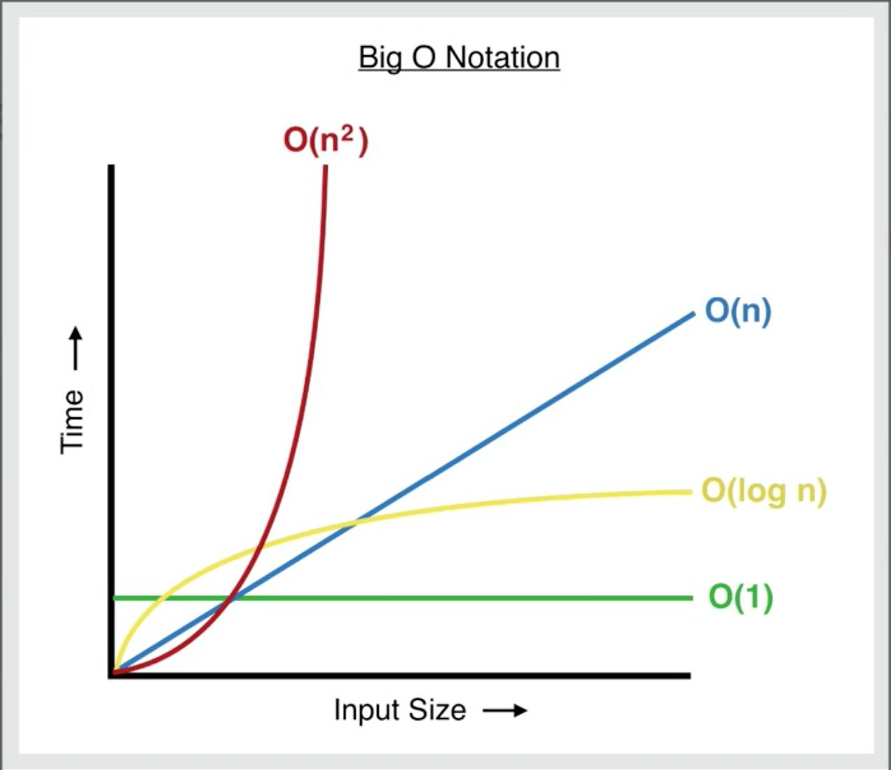
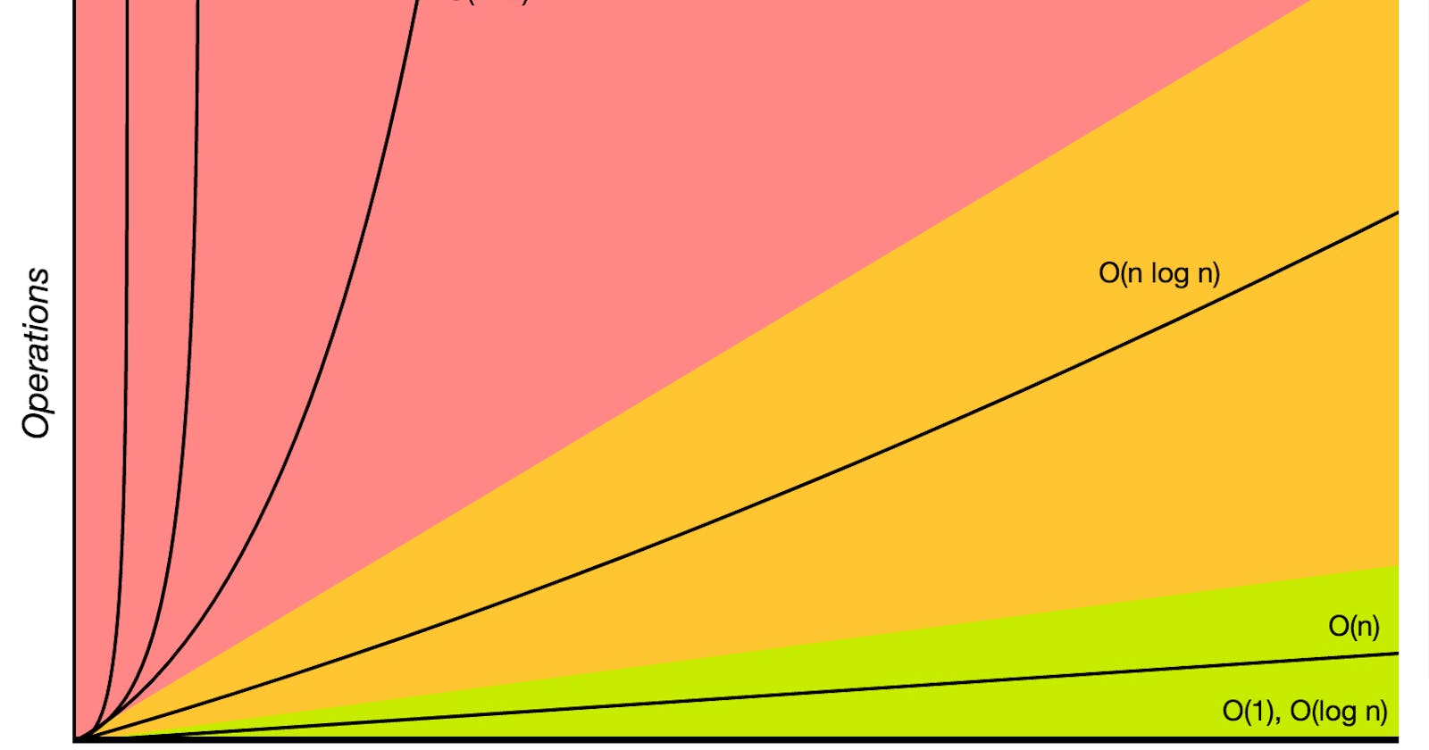
Big-O notation is the terminology we use to describe how long it takes an algorithm to execute (time complexity) or how much storage in memory or on disk the algorithm requires (space complexity). Big-O notation can be used to indicate the optimal, worst, and average cases of an algorithm's time and space complexity. As a software developer, you'll notice that most Big-O discussions center on an algorithm's worst-case running time.
It is crucial to remember that "running time" in Big-O notation does not immediately equal to time as we understand it e.g. seconds, milliseconds, microseconds, etc. Big-O notation, instead, measures how fast the runtime increases in proportion to the size of the input. Thus, it follows that the term "time complexity" refers to how we evaluate an algorithm's runtime as the number of its inputs grows and space complexity refers to how we evaluate the amount of extra memory required to run the code in our algorithm. As a result, Big-O notation is used to rate algorithms based on how well they work with huge inputs.
It is important to understand the Big-O notation because, in many programming languages, there are numerous ways of doing the same operation. So, in order to discuss tradeoffs between techniques and identify flaws in your code, we utilize Big-O notation. This is because, by understanding time and space complexity, you will have a better understanding of the idea of efficiency and will be able to identify bottlenecks in your code that should be fixed, especially when working with large data sets.
How can we compute Big-O of Time Complexity?
To put it simply, we count the number of basic operations that the computer must complete. This makes much more sense than timing the code itself using built-in timers because various computers' execution times might vary, and this is not an accurate estimate of the code's runtime. When we count basic operations, the number remains constant regardless of the machine we're using. A particular algorithm's time complexity can be categorized into one of the following categories (in increasing order of complexity):
1. Constant Time O(1)
O(1) denotes that an algorithm takes a constant amount of time to run, regardless of the quantity of the input.
Bookmarks are an excellent example of how constant time might manifest itself in the "real world." Bookmarks allow a reader to quickly find the last page that they read. It makes no difference whether you're reading a book with 30 pages or a book with 1000 pages. If you're using a bookmark, you'll be able to find the final page in a single step. Many operations in computer programming are constant-time. Following are some examples:
a) operations in mathematics
b) using the index to retrieve an array
c) gaining access to a hash using the key
c)pushing and popping on a stack
d) inserting and removing from a queue
d) returning a value from a function
For example:
if a > b:
    return True
else:
    return False
2. Logarithmic Time O(log n)
O(log n) denotes that the running time rises in proportion to the logarithm of the input size, implying that the run time rarely increases as the input size grows exponentially.
Example 1
Consider a classroom of 400 pupils in which you only gave one individual your pen. You want that pen now. to do this in logarithmic time, you would divide the students into two groups, then ask: “Is it on the left side, or the right side of the classroom?” Then divide that group in half and ask again, and so on. you would repeat this process until you only have one pupil left who possesses your pen. This is what you mean when you say O (log n).
Example 2
Finding a word/phrase in a physical dictionary by reducing my sample size by half at each step exemplifies how logarithmic time works in the "real world." For example, when looking for the word "photograph" I could open the dictionary exactly in the center, at which time I could establish if terms beginning with "p" occur before or after the words I'm presently examining. I can disregard all of the pages in the first half of the book after I've determined that "p" is in the second half of the book. I then go through the same steps again. Following this approach all the way to the finish would cut the number of pages I have to search through in half every time till I located the word.
In programming, a binary search operation is the most commonly used example when discussing logarithmic run times.
3. Linear Time O(n)
O(n) denotes that the run time grows at the same rate as the input. Reading a book is an illustration of how linear time might behave in the "real world." Assume that reading a single page of a big print book takes me precisely one minute. Given that, a 30-page book will take me 30 minutes to read. Similarly, a book with 1000 pages equals 1000 minutes of reading time. In the pen example above, this would entail walking around to each of the 400 pupils and asking them personally whether they have your pen.
One of the most popular linear-time operations in programming is traversing an array. For example:
for value in data:
    print(value)
4. Quadratic Time O(n^2)
O(N2) denotes an algorithm whose performance is exactly proportional to the square of the input data set size. When an algorithm must execute a linear time operation for each value in the input data, it is said to have a quadratic time complexity. Deeper nested iterations will provide O(N^3), O(N^4), and so on. In general- but not always, finding two nested loops is a good sign that the piece of code you're looking at has an O(n^2) execution time. Similarly, three stacked loops would represent an O(n^3) execution time and so on. for example:
for x in data:
    for y in data:
        print(x, y)
In programming, Many of the most fundamental sorting algorithms such as Bubble Sort, Insertion Sort, and Selection Sort have a worst-case execution time of O(n^2)
N/B: O(n log n), which is sometimes misunderstood with O(log n), denotes that an algorithm's running time is log-linear, which is a mix of linear and logarithmic complexity. Sorting algorithms that use a divide and conquer method, such as merge sort, timsort, and heapsort are log-linear.
5. Factorial Time O(n!)
When an algorithm expands in a factorial manner dependent on the size of the input data, it is said to have a factorial time complexity, for example:
2! = 2 x 1 = 2
3! = 3 x 2 x 1 = 6
4! = 4 x 3 x 2 x 1 = 24
5! = 5 x 4 x 3 x 2 x 1 = 120
6! = 6 x 5 x 4 x 3 x 2 x 1 = 720
7! = 7 x 6 x 5 x 4 x 3 x 2 x 1 = 5.040
8! = 8 x 7 x 6 x 5 x 4 x 3 x 2 x 1 = 40.320
As you can see, it expands quite quickly, even with a modest size input. The Heap's algorithm, which is used to generate all conceivable permutations of n items, is an excellent example of a factorial time complexity algorithm.

Big-O Calculation
When calculating Big-O, remember the following:
- Remove the Constants
- Drop the Non-Dominant Terms
For example:
def my_function(data):
# The segment below executes in O(1)
    first_element = data[0]

# The segment below executes in O(n)
    for value in data:
        print(value)

# The segment below executes in O(n^2)
    for x in data:
        for y in data:
            print(x, y)
Despite the fact that the operations in 'my function' are illogical, we can observe that it has various time complexities: O(1) + O(n) + O(n^2). As the size of the input data increases, the operation that takes O(n^2) will become the bottleneck of this method. Based on this, we may define the algorithm's time complexity as O(n^2).
